Examples and Tutorial Guide
This section was created with the purpose of providing a comprehensive example that covers the main functions of the Phybers package. Here, you will find well-commented test codes and data that will allow you to explore many functionalities of the package.
To make the examples more comprehensive, we start with the How to calculate tractography data from diffusion-weighted images using DSI Studio software subsection,
where we describe how to calculate brain tractography data using the DSI Studio software [1].
We also provide a source code that allows you to convert a tractography dataset from TRK (used by DSI Studio, TrackVis, among others)
or TCK (used by MRtrix and others) formats to the bundles format, and vice versa.
Then, in the Examples of Phybers use subsection, we provide test data for running each of the showcased examples, divided into Fiber segmentation and visualization example and Clustering example.
It’s important to note that completing the How to calculate tractography data from diffusion-weighted images using DSI Studio software subsection is not necessary to try the provided examples.
You can start directly in the Test data download subsection to run them. Additionally, for detailed documentation on each Phybers module, we recommend accessing the Documentation section.
How to calculate tractography data from diffusion-weighted images using DSI Studio software
Currently, various programs enable the calculation of brain tractography.
Nevertheless, in this subsection, we suggest a workflow to obtain a brain tractography dataset from diffusion MRI data of a subject of the Human Connectome Project (HCP) database [2],
utilizing DSI Studio software [1].
Furthermore, we also tested and provide examples for dMRI data of a subject from the OpenNeuro MRI Database,
wich has a lower resolution than the HCP database. The example data is compatible with all phybers modules.
To increase usability, we provide a code to convert the brain tractography dataset file from the output format of DSI Studio (TRK) to our working format (bundles).
This code source is also employed for converting from the TCK format to the bundles format, ensuring compatibility with other programs such as MRtrix, among others.
Download and install the DSI Studio software by following the instructions provided on the DSI Studio website.
HCP database
The Human Connectome Project (HCP) has made available a freely accessible high-quality brain imaging database. The images were acquired on a 3 Tesla Siemens Skyra scanner. Multi-shell diffusion data was collected with three b-values (1000, 2000, 3000 \(s/mm^{2}\)), 270 diffusion weighting directions, and an isotropic voxel size of 1.25 mm.
To perform tractography, use preprocessed diffusion MRI images from an HCP subject, which can be downloaded from the following website:
HCP ConnectomeDB.
You can also download an example scan from here.
When you obtain the example scan, unzip the file ('subject_diffusion_MRI_example.zip') using the extract here option.
Diffusion MRI data processed through the HCP diffusion pipeline includes diffusion MRI images ('data.nii.gz'), b-values (bvals), directions (bvecs),
a brain mask ('nodif_brain_mask.nii.gz'), a file ('grad_dev.nii.gz') that can be utilized to address gradient nonlinearities during model fitting,
and log files detailing the EDDY processing (found in the 'subject_diffusion_MRI_example/eddylogs/' directory).
Afterward, you have the option to compute whole-brain tractography with DSI Studio. This can be done through the graphical interface or by using command lines. For a single subject, we suggest performing it through the graphical user interface. Open the graphical user interface and follow the subsequent 3 steps (Figure 1):
Step T1: Open Source Images: allows reading diffusion MRI images in
NIfTIorDICOMformat and then creating theSRCfile. In this case, the diffusion MRI images are located in the file'data.nii.gz'.Step T2: Reconstruction: the
SRCfile is read. Subsequently, skull stripping techniques or opening a brain mask ('nodif_brain_mask.nii.gz') can be applied. Eddy current and motion corrections are then applied. Afterward, the diffusion reconstruction method is selected, with GQI being the chosen method in this case. Finally, theFIBfile is generated.Step T3: Fiber Tracking & Visualization: takes the
FIBfile and allows you to adjust parameters for fiber tracking. In this case, you can perform whole-brain deterministic tractography with the following fiber tracking parameters: angular threshold = \(60^{0}\), step size = 0.5 mm, smoothing = 0.5, minimum length = 30 mm, maximum length = 300 mm, and a tract count of 1.5 million fibers. To conclude, the tractography dataset can be stored inTRKformat.
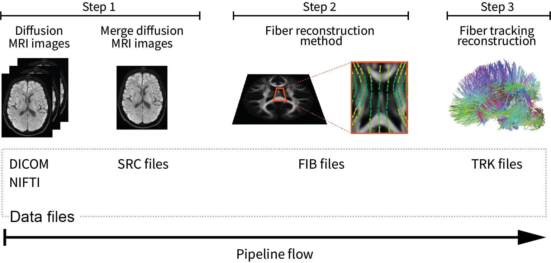
Figure 1. Workflow suggested to generate a whole-brain tractography dataset in DSI Studio for testing.
In Step T1, diffusion MRI images are read from NIfTI or DICOM format, and create SRC file.
Step T2 involves applying motion and distortion corrections, selecting the diffusion reconstruction method, ultimately leading to the creation of the 'FIB' file
Step T3, enables fiber tracking and the saving of the tractography dataset in TRK format.
OpenNeuro database
Alternatively, you can obtain a brain tractography dataset using lower-resolution diffusion MRI images. For example, on the OpenNeuro website, you can download diffusion images from 25 subjects. OpenNeuro has provided an open-access brain imaging database. The scans were performed on a 1.5 Tesla Philips Intera MRI scanner. Diffusion-weighted images were acquired using a single-shot echo-planar imaging sequence with 15 non-collinear and non-coplanar diffusion weighting directions, and b-values of 0 (b0 image) and 1000 \(s/mm^{2}\). The voxel size is 2x2x3 mm.
We have taken a subject from OpenNeuro and made it available at the following link.
Download the subject to the 'Downloads/' directory and unzip it using the extract here option.
Then, check for the existence of the three necessary files for tractography calculation: diffusion MRI images ('data_openneuro.nii.gz')
and the respective directions and b-values ('data_openneuro.bvec', 'data_openneuro.bval').
Subsequently, you can use DSI Studio software to calculate brain tractography and follow the same steps described above.
We recommend using the DTI fiber reconstruction method with the following tracking parameters:
angular threshold = \(60^{0}\), step size = 1.0 mm, smoothing = 0.5, minimum length = 30 mm,
maximum length = 250 mm, and a tract count of 1.0 million fibers.
Conversion of tractography data to working format (TRK or TCK -> bundles)
To ensure compatibility of our working format (bundles) with other software (DSI Studio, Dipy, MRtrix, among others), we offer a source code for performing format conversions.
The following code allows you to convert tractography dataset from the TRK or TCK formats (obtained with DSI Studio) to the bundles format.
In the next subsection, we provide code for converting from bundles format to TRK or TKC.
To test this code, download the test dataset to the 'Downloads/' directory on your computer and
then unzip it with the extract here option.
In the 'Downloads/format_conversion_testing/' directory you will find three files. The files 'tractography_format_test.trk' and 'tractography_format_test.tck',
containing 10K brain fibers, in TRK and TCK formats, respectively.
The file 'diffusion_data.nii' is the diffusion MRI image in the diffusion-weighted subject’s acquisition space.
This image is used to extract the voxel size and the number of slices necessary to apply the affine transformation and convert the tractography dataset from one format to another.
Next, within the 'Downloads/format_conversion_testing/' directory, create a text file named 'format_conversion_tool.py', copy the following code, and save it.
# Import for enabling parallel processing:
from joblib import Parallel, delayed

# Import of the nibabel library for handling image file:
import nibabel as nb

# Import of the NumPy library:
import numpy as np

# Import necessary modules from Phybers for writing fiber bundles:
from phybers.utils import write_bundle, read_bundle

# Import necessary functions for loading and saving tractograms from Dipy library:
from dipy.io.streamline import load_tractogram, save_tractogram

# Import necessary classes for handling stateful tractograms and specifying coordinate space from Dipy library:
from dipy.io.stateful_tractogram import Space, StatefulTractogram

def apply_affine_bundle_parallel(in_fibers, affine, nthreads):
   """Use parallel processing to apply the affine transformation to each fiber.
   """
   # Use parallel processing to apply the affine transformation to each fiber:
   out_fibers = Parallel(n_jobs=nthreads)(delayed(apply_affine_fiber)(f, affine) for f in in_fibers)

   return out_fibers

def apply_affine_point(in_point, affine):
   """Apply an affine transformation to a 3D point.
   """
   # Apply the affine transformation to the input point:
   tmp = affine * np.transpose(np.matrix(np.append(in_point, 1)))

   # Extract the transformed point coordinates
   out_point = np.squeeze(np.asarray(tmp))[0:3]

   return out_point

def get_affine(image_reference):
   """ Get an affine transformation matrix from an image reference.
   """
   # Load the image reference:
   img_reference = nb.load(image_reference)

   # Get the affine transformation matrix from the image reference:
   affine_ = img_reference.affine

   # Ensure all values in the affine matrix are positive:
   affine_ = np.abs(affine_)

   # Apply specific modifications to the diagonal elements and translation vector:
   affine_[0, 0] = -1
   affine_[1, 1] = -1
   affine_[2, 2] = -1
   affine_[0:3, 3] = np.array(img_reference.header.get_zooms()) * np.array(img_reference.header.get_data_shape())

   return affine_

def apply_affine_fiber(fiber, affine):
   """Apply an affine transformation to a fiber.
   """
   new_fiber = []

   # Apply the affine transformation to each point in the fiber:
   for p in fiber:
      point_transform = apply_affine_point(p, affine)
      new_fiber.append((point_transform))

   return np.asarray(new_fiber, dtype=np.float32)

def convert_to_bundles(file_in = '', image_reference = '', file_out_name = ''):
   """Convert streamlines from TRK or TCK format to bundles format.
   """
   # Get the affine transformation matrix:
   affine = get_affine(image_reference)

   # Load the streamlines from file:
   fibers = nb.streamlines.load(file_in).streamlines

   # Apply the affine transformation to the streamlines in parallel:
   fibers_converted = apply_affine_bundle_parallel(fibers, affine, -1)

   # Write the streamline to bundles format:
   write_bundle(f'{file_out_name}.bundles', fibers_converted)
Now, to convert from TRK to bundles format, at the end of the script 'format_conversion_tool.py', add the following lines:
# Input reference image file:
image_reference = 'diffusion_data.nii'

# Input tractography dataset file in TRK format:
file_in= 'tractography_format_test.trk'

# Output tractography dataset file name to convert in bundles format:
file_out_name = 'tractography_bundles_from_trk'

# # Execute the function to convert the TRK format to bundle:
convert_to_bundles(file_in, image_reference, file_out_name)
Subsequently, run the code to obtain the converted fibers in the bundles format. In the directory 'Downloads/format_conversion_testing/',
you can verify that the fibers were converted, if the following two files are created:
'tractography_format_test_trk.bundles' and 'tractography_format_test_trk.bundlesdata'.
To convert from TCK to bundles format, follow the same procedure, but in this case, use file_in = 'tractography_format_test.tck'.
Conversion of tractography data from working format to other formats (bundles -> TRK or TCK)
This subsection introduces a code for converting from the bundles format to TRK and TCK formats.
To employ this code, insert the following function into the script 'format_conversion_tool.py' and save afterward.
def convert_bundles_to_track(file_in = '', image_reference = '', file_out_name = '', format_out = ''):
   """ Convert streamlines from bundles format to TRK or TCK formats.
   """

   # Load the reference NIfTI image
   nifti_img = nb.load(image_reference)

   # Read tractography dataset from the input file:
   fibers = read_bundle(file_in)

   # Initialize an empty list to store transformed fibers:
   fibs = []

   # Iterate through each fiber in the input tractography dataset:
   for i in range(len(fibers)):
      fib = fibers[i]

      # Initialize an array with zeros to store transformed fiber points:
      fib2 = np.zeros_like(fib)

      # Iterate through each point in the fiber:
      for j in range(len(fib)):

            # Transform each point by subtracting it from the data shape of the NIfTI image:
            fib2[j, 0] = np.array(nifti_img.header.get_data_shape())[0] - fib[j][0]
            fib2[j, 1] = np.array(nifti_img.header.get_data_shape())[1] - fib[j][1]
            fib2[j, 2] = np.array(nifti_img.header.get_data_shape())[2] - fib[j][2]

      # Append the transformed fiber to the list:
      fibs.append(fib2)

   # Create an identity affine matrix:
   affine_ = np.eye(4)

   # Create a NIfTI image from the reference image data:
   nifti_img_ref = nb.Nifti1Image(nifti_img.get_fdata(), affine_)

   # Create a stateful tractogram using transformed fibers and the reference NIfTI image:
   tractogram = StatefulTractogram(fibs, nifti_img_ref, Space.VOX)

   # Save the stateful tractogram as a TRK file:
   save_tractogram(tractogram, file_out_name + '.' + format_out, bbox_valid_check=False)
Below is an example for converting from the bundles format to TRK. Refer to the script 'Downloads/format_conversion_testing/format_conversion_tool.py',
and at the end of the script, add the following lines that execute the convert_bundles_to_track() function.
Then, verify that the file 'tractography_trk_from_bundles.trk' has been created in the 'Downloads/format_conversion_testing' directory.
# Input reference image file:
image_reference = 'diffusion_data.nii'

# Input tractography dataset file in bundles format:
file_in = 'tractography_bundles_from_trk.bundles'

# Output tractography dataset file name to convert:
file_out_name = 'tractography_trk_from_bundles'

# Output chosen format for conversion to the input tractography dataset file:
format_out = 'trk'

# Execute the function to convert the bundles format to TRK::
convert_bundles_to_track(file_in, image_reference, file_out_name, format_out)
Examples of Phybers use
This subsection provides all the necessary test data to run the main functionalities of Phybers. Two main examples, Fiber segmentation and visualization example and Clustering example have been created for this purpose.
The first step would be to obtain the test data from Test data download,
and then you can run both examples in any order you prefer, as each one is independent from the other.
In the Fiber segmentation and visualization example, an illustration is given of how the Utils module (deform(), sampling(),
and intersection()) and the Visualization module (start_fibervis()) integrate with tractography segmentation using the fiberseg() algorithm.
In the Clustering example, an integrative example is presented that allows combining the Utils module (postprocessing()) and
the Visualization module (start_fibervis()) with the clustering module’s algorithms hclust() and ffclust().
Additionally, an example is provided to analyze clustering results, such as obtaining a histogram of clusters with a size greater than 150 (fibers) and a length between 50 and 60 mm.
Test data download
For the execution of all Phybers functions, two sets of diffusion MRI testing data are available. The initial set features higher-resolution data sourced from the HPC database, while the second set is derived from a lower-resolution dataset from the OpenNeuro database. The example scripts provided here were created using higher-resolution data, but instructions are given to apply them to the second database.
To run each of the examples provided below, download the HCP dataset
to the 'Downloads/' directory on your computer,
and then unzip the data using the extract here option. This will generate the 'Downloads/testing_phybers/' directory, which should contain:
a NIfTI image with the nonlinear transformation to deform the tractography dataset to the MNI space ('nonlinear_transform.nii'),
and two files of brain tractography datasets with their respective bundles/bundlesdata files. These datasets are named 'subject_15e5.bundles/subject_15e5.bundlesdata'
and 'subject_4K.bundles/subject_4K.bundlesdata'.
Both tractography datasets correspond to the same test subject; their fibers have a variable number of points and are aligned with the subject’s diffusion-weigthed acquisition space.
The first tractography dataset has a size of 1.5 million ('15e5') brain fibers from the whole-brain, while the second dataset has 4,000 ('4K') brain fibers from the postcentral region of the brain.
Next, execute the following examples within the 'Downloads/testing_phybers/' directory.
To access the OpenNeuro database data in a format compatible for direct use with Phybers, we invite you to download it through the
provided link.
Follow the same download and decompression steps as outlined for the HCP dataset.
Subsequently, verify the presence of the following files within the directory 'Downloads/testing_phybers_OpenNeuro_database/'.
'subject_openneuro_1M.bundes/subject_openneuro_1M.bundesdata' contains the whole-brain tractography dataset, aligned with the subject’s diffusion-weighted acquisition space,
featuring a size of 1 million ('1M') brain fibers.
'nonlinear_transform_oepnneuro.nii' has the nonlinear transformation to deform the tractography dataset to the MNI space.
Finally, 'subject_openneuro_4K.bundes/subject_openneuro_4K.bundesdata'
has brain fibers from the postcentral region of the brain, aligned with the subject’s diffusion-weighted acquisition space, featuring a size of 4,000 ('4K') brain fibers.
Fiber segmentation and visualization example
Fiber bundle segmentation
To perform the fiber bundle segmentation, it is crucial that the subject’s tractography dataset has fibers resampled with 21 equidistant points and is in the same space as the brain fiber bundle atlas.
To carry out the segmentation example, follow these three steps:
First, download the test data detailed in the previous subsection Test data download.
Second, download the Deep White Matter (DWM) bundle atlas (Guevara et al. 2012) as described in the subsection
Atlases Download, to the 'Downloads/testing_phybers/' directory and then unzip it with the extract here option.
You can also use either of the other two Superficial White Matter (SWM) atlases provided in the subsection Atlases Download.
Third, create a script file with the name 'testing_fiberseg.py', copy the following command lines, save,
and execute the script in a Python terminal within the 'Downloads/testing_phybers/' directory.
# Import Python's os library for directory management:
import os

# Import deform  sub-module. Transforms a tractography dataset file to another space using a nonlinear deformation image file:
from phybers.utils import deform

# Import sampling  sub-module. Performs a sampling of the fibers points:
from phybers.utils import sampling

# Import fiberseg sub-module. White matter fiber bundle segmentation algorithm based on a multi-subject atlas:
from phybers.segment import fiberseg

#Execute the deform function:
deform ( deform_file = 'nonlinear_transform.nii', file_in = 'subject_15e5.bundles', file_out = 'subject_15e5_MNI.bundles')

# Execute the sampling function:
sampling ( file_in = 'subject_15e5_MNI.bundles', file_out = 'subject_15e5_MNI_21pts.bundles', npoints = 21 )

# Path to the tractography dataset file:
file_in = 'subject_15e5_MNI_21pts.bundles'

# Subject name used to label the results; in this case, the suffix 'subject_15e5' is used:
subj_name = 'subject_15e5'

# Directory to the bundle atlas:
atlas_dir = os.path.join('DWM_atlas_2012','bundles')

# Path to the atlas information file:
atlas_info = os.path.join('DWM_atlas_2012','atlas_info.txt')

# Directory to save all result segmentation, in this case 'seg_result':
dir_out = 'seg_result'

# Execute the fiberseg function:
fiberseg(file_in, subj_name, atlas_dir, atlas_info, dir_out)
The first step to verify that the segmentation was performed correctly would be to open the 'Downloads/testing_phybers/seg_result/' directory and check that the following 3 directories were created:
'Downloads/testing_phybers/seg_result/final_bundles/': It contains separately all the segmented fascicles inbundles/bundlesdatafiles, sampled at 21 points and in the atlas space (MNI). For example, for the inferior longitudinal fascicle (IL), we should find two files:'subject_15e5_to_IL_LEFT_MNI.bundles'and'subject_15e5_to_IL_LEFT_MNI.bundlesdata'. The names encode that we are dealing with the segmentation result for the subject'subject_15e5', specifically for the inferior longitudinal fascicle in the left hemisphere ('IL_LEFT'), and it is located in the MNI space. This convention holds for the rest of the fascicles.'Downloads/testing_phybers/seg_result/bundles_id/': It is a directory that has a text file for each segmented bundle. A text file of a segmented bundle contains the indices of the fibers in the original subject’s tractography dataset file. The name of each file corresponds to the name of the segmented bundle file with a'.txt'extension. These files are used to obtain the segmented fascicles in the subject’s original space and with all points of brain fibers.'Downloads/testing_phybers/seg_result/centroids/': A directory storing two files corresponding to a tractography dataset inbundles/bundlesdataformat, containing one centroid for each segmented fascicle. This dataset is named'centroids.bundles/centroids.bundlesdata', and is sampled at 21 points in the atlas space (MNI).
Visualization of segmented fascicles
The second step to check the segmentation results would be to use our visualization software to observe the segmented fascicles.
To do this, execute the following commands in the 'Downloads/testing_phybers/' directory:
# Import fibervis:
from phybers.fibervis import start_fibervis

# Execute the graphical user interface for fibervis:
start_fibervis()
Subsequently, navigate to the directory that stores all segmented bundles, in this case, 'Downloads/testing_phybers/seg_result/final_bundles/'.
As example, select the 3 segments of the arcuate fasciculus (AR) for the left hemisphere: 'subject_15e5_to_AR_LEFT_MNI.bundles',
'subject_15e5_to_AR_ANT_LEFT_MNI.bundles', and 'subject_15e5_to_AR_POST_LEFT_MNI.bundles' .
This will allow you to obtain a visualization similar to the one shown in Figure 2.
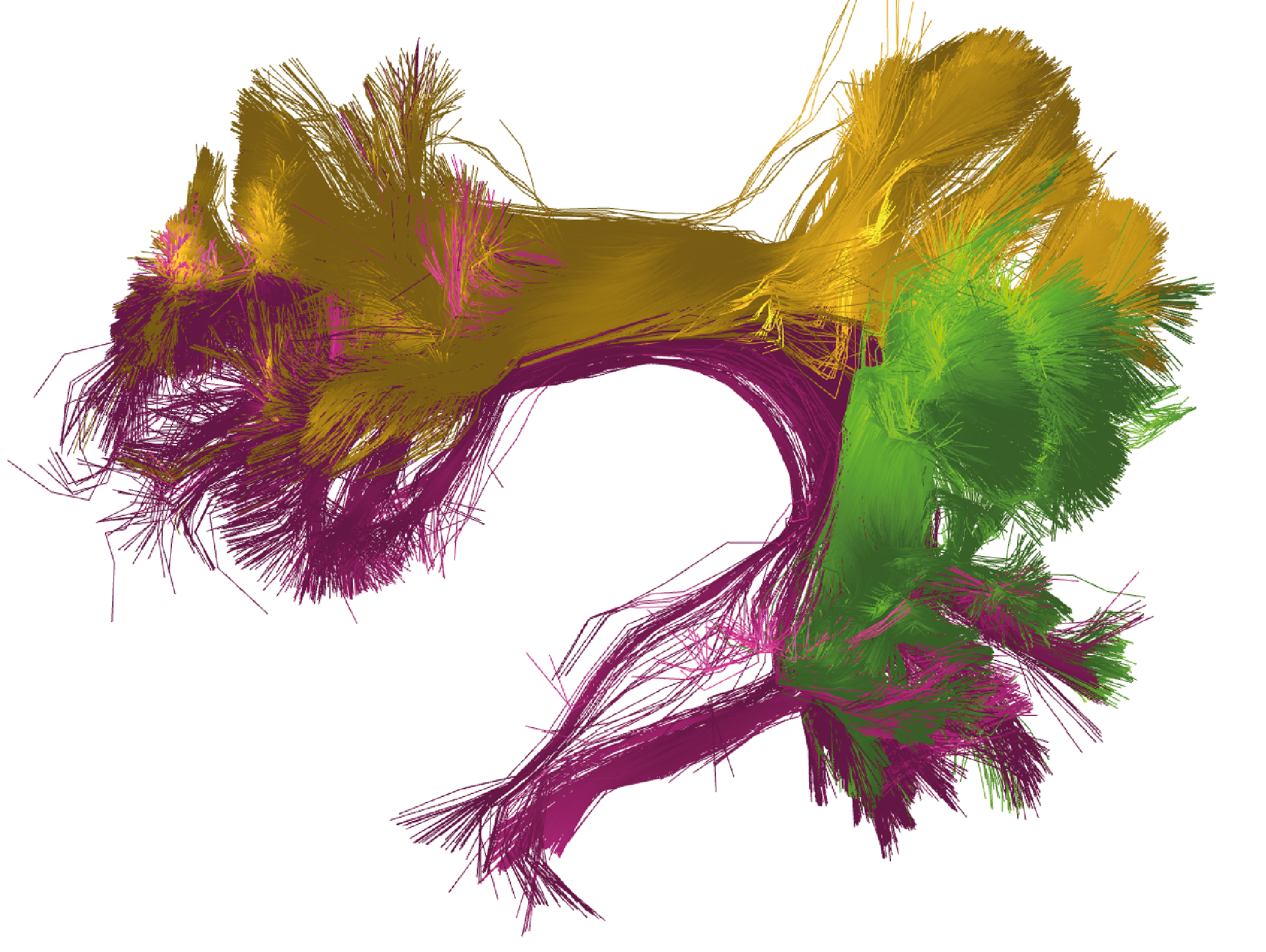
Figure 2. Bundle segmentation results for a subject from the HCP database using the DWM bundle atlas [3]. The three segments of the arcuate fasciculus in the left hemisphere: direct segment (purple), anterior segment (yellow), and posterior segment (green). Colors are randomly assigned.
Alternatively, you can execute the segmentation example using the brain tractography dataset from OpenNeuro (Test data download), and use it with file_in ='subject_openneuro_1M.bundes'.
In this case, we recommend adjusting the segmentation
thresholds for each of the fascicles in the DWM bundle atlas or simply download and replace the atlas information file ('atlas_info.txt') we provided at the
following link.
Figure 3 visualizes the segmentation results for the three segments of the arcuate fascicle.
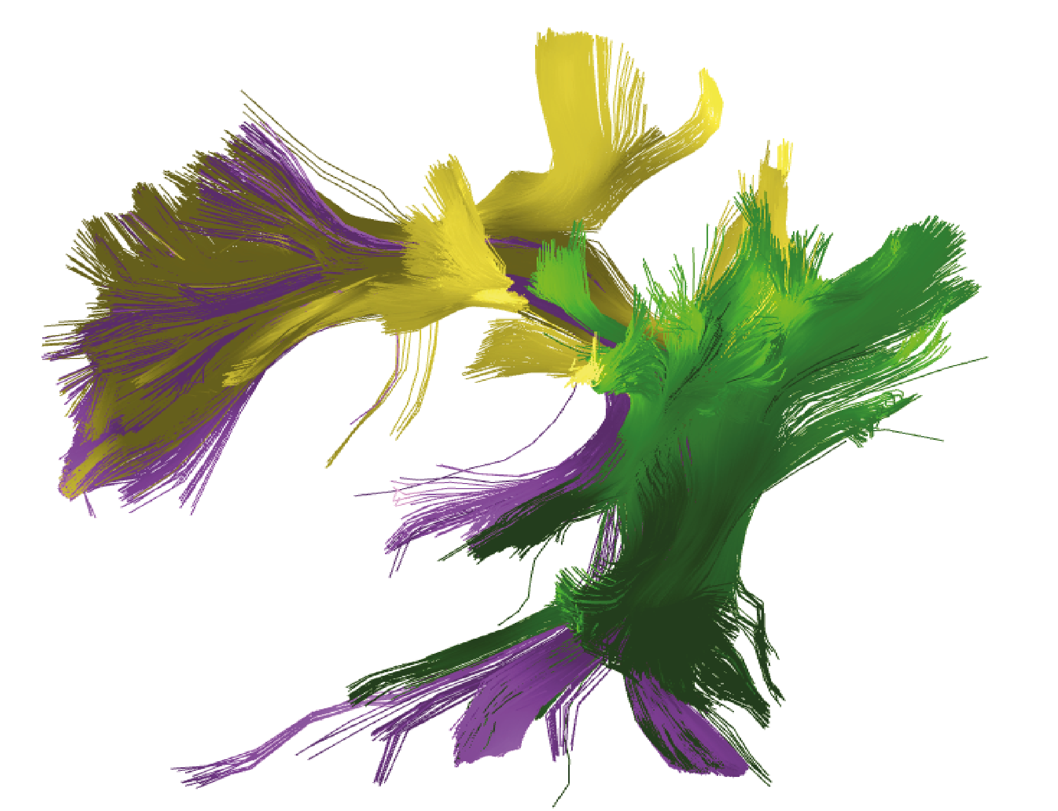
Figure 3. Bundle segmentation results for a subject from the OpenNeuro database using the DWM bundle atlas [3]. The three segments of the arcuate fasciculus in the left hemisphere: direct segment (violet), anterior segment (yellow), and posterior segment (green). Colors are randomly assigned.
Retrieve the fascicles with all points in the subject’s original space
In the 'Downloads/testing_phybers/seg_result/final_bundles/' directory, all fascicles identified in the test subject are stored.
These fascicles have the same number of fiber points, specifically, 21 points, and are located in the atlas space.
In case you need to obtain the fascicles in original space, where the bundles were tracked (usually the subject’s diffusion-weighted space)
and with the same number of points as the original tractography dataset, execute the following commands on the 'Downloads/testing_phybers/' directory.
This will generate a new directory inside 'Downloads/testing_phybers/seg_result/' called 'final_bundles_allpoints'.
# Import Python libraries for additional processing steps:
import os
import numpy as np

# Import necessary Phybers modules for fiber reading and writing, respectively:
from phybers.utils import read_bundle, write_bundle

# Read the fibers with all points and in the subject's original space:
bundles_allpoint = read_bundle('subject_15e5.bundles')

# Convert the bundle list into a NumPy array
bundles_allpoint_to_array = np.asarray(bundles_allpoint, dtype=object)

# Create a directory to store the final bundles with all points
directory = os.path.join('seg_result', 'final_bundles_allpoints')
if not os.path.exists(directory):
   os.mkdir(directory)

# Iterate through files in the 'bundles_id/bundles_id' directory
for file_id in os.listdir(os.path.join('seg_result', 'bundles_id')):
   indices=[]

   # Read indices from the file
   with open(os.path.join('seg_result', 'bundles_id',file_id), 'r') as f:
      for line in f:
            indices.append(int(float(line.strip())))

   # Write the fibers with all points to a new bundle file
   write_bundle(os.path.join('seg_result','final_bundles_allpoints',file_id[:-4]+'.bundles'),bundles_allpoint_to_array[indices])
Calculating intersection between fascicles
The phybers.utils module includes the intersection tool, designed to calculate the percentage of overlap between two given fascicles.
To consider two fibers as intersecting, their maximum Euclidean distance must be less than a defined threshold, given as a parameter (distance_thr) with a default value of 10.0 mm.
This function can be used to compare fascicles from different processing, for example,
for evaluating the impact of linear versus nonlinear registration on segmented data, as outlined in Román et al. [4].
Additionally, it can be employed to identify similarities between the same fascicle across two different subjects.
In this example, we propose computing the intersection of the segmented left anterior arcuate fasciculus in MNI space ('subject_15e5_to_AR_ANT_LEFT_MNI.bundles')
with the segmented left direct arcuate fasciculus in MNI space ('subject_15e5_to_AR_LEFT_MNI.bundles'). Then, we can proceed with the bundle intersection calculation (phybers.utils.intersection()).
Thus, the fascicle 'subject_15e5_to_AR_ANT_LEFT_MNI.bundles' will be passed to the file1_in argument, while 'subject_15e5_to_AR_LEFT_MNI.bundles' will be passed to the file2_in argument.
Additionally, the output directory name will be set to the dir_out argument, in this case:
'Downloads/testing_phybers/seg_result/intersection_output/'.
The intersection function returns a tuple with the percentage of intersection of the first bundle with the second and vice versa. Also, the function generates three tractography dataset files in the ouput directory, as follows:
'fiber1-fiber2.bundles/fiber1-fiber2.bundlesdata': containing the fibers that are considered similar (or intersecting) for both fascicles.'only_fiber1.bundles/only_fiber1.bundlesdata': containing the fibers that are only in the first fascicle.'only_fiber2.bundles/only_fiber2.bundlesdata': containing the fibers that are only in the second fascicle.
Open a Python terminal in the 'Downloads/testing_phybers/' directory and run the following commands:
# Import intersection sub-module:
from phybers.utils import intersection

# Import Python's os library for directory management:
import os

# Execute the intersection function:
result_intersection = intersection(file1_in = os.path.join('seg_result', 'final_bundles', 'subject_15e5_to_AR_ANT_LEFT_MNI.bundles'),
                                 file2_in = os.path.join('seg_result', 'final_bundles', 'subject_15e5_to_AR_LEFT_MNI.bundles'),
                                 dir_out = os.path.join('seg_result', 'intersection_output'), distance_thr = 40)

# Display the results of intersection
print('Intersection fibers1 with fibers2 ', result_intersection [0])
print('Intersection fibers2 with fibers1 ', result_intersection [1])
In Figure 4, the left side displays the overlap of the 'only_fiber1.bundles' fascicle with the 'fiber1-fiber2.bundles' fibers,
while the right side shows the 'only_fiber2.bundles' fascicle with the 'fiber1-fiber2.bundles' fibers.
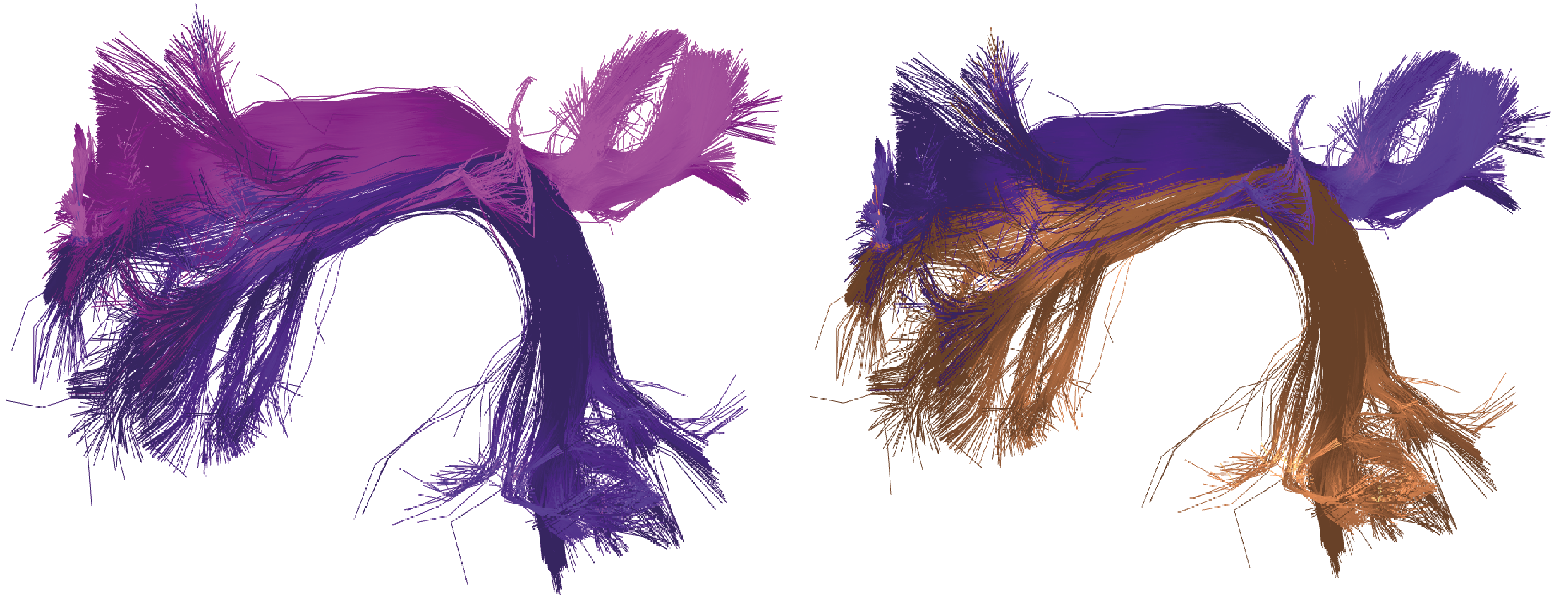
Figure 4. Example of intersection between the left anterior arcuate fasciculus (first fascicle) and the left direct arcuate fasciculus (second fascicle), both obtained in the segmentation example. On the left, the overlap of fibers intersecting in both fascicles is shown: fibers from the first fascicle are represented in pink, and intersecting fibers from the second fascicle are in violet. On the right, the intersecting fibers from both fascicles are presented, with those belonging to the second fascicle highlighted in brown and those from the first fascicle that intersect, in violet.
Clustering example
The clustering module includes two clustering algorithms: HClust and FFClust.
First, an example of how to apply HClust ('phybers.clustering.hclust()') will be presented, followed by an example of FFClust use ('phybers.clustering.ffclust()').
Before carrying out any of the provided examples, download the test data following the instructions given in section Test data download.
HClust
Navigate to the 'Downloads/testing_phybers/' directory, open a Python terminal, and execute the commands provided below.
# Import hclust sub-module. Average-link hierarchical agglomerative clustering algorithm:
from phybers.clustering import hclust

# Path to the tractography dataset file:
file_in = 'subject_4K.bundles'

# Directory to save all result clustering:
dir_out = 'hclust_result'

# Maximum distance threshold in mm:
fiber_thr = 70

# Adaptive partition threshold in mm:
partition_thr = 70

# Variance squared and provides a similarity scale in mm:
variance = 3600

# Execute the hclust function:
hclust(file_in, dir_out, fiber_thr, partition_thr, variance)
If HClust was executed successfully, in the directory 'Downloads/testing_phybers/hclust_result/' you should be able to verify the existence of the following outputs:
'Downloads/testing_phybers/hclust_result/final_bundles/': Directory that stores all the fiber clusters identified in separated datasets (bundles/bundlesdatafiles), sampled at 21 points. The file names are labeled with integer numbers ranging from zero to the total number of fiber clusters (N-1) identified.'Downloads/testing_phybers/hclust_result/final_bundles_allpoints/': Directory that stores all the fiber clusters identified in separated datasets (bundles/bundlesdatafiles), with all points and in the original space. The file names are labeled with integer numbers ranging from zero to the total number of fiber clusters (N-1) identified.'Downloads/testing_phybers/hclust_result/centroids/': A directory storing two files corresponding to a tractography dataset inbundles/bundlesdataformat, containing one centroid for each created cluster. This dataset is named'centroids.bundles/centroids.bundlesdata', and is sampled at 21 points in the atlas space (MNI).'Downloads/testing_phybers/hclust_result/bundles_id.txt': Text file that stores the fiber indexes from the original input tractography dataset file for each detected cluster. Each line in the file correspond to a cluster in correlative order.'Downloads/testing_phybers/hclust_result/outputs/': Temporal directory with intermediate results, such as the distance matrix, the affinity graph, and the dendrogram.
Visualization of the clusters obtained with HClust
Additionally, you can use the visualization module to observe and interact with the obtained results for HClust.
First, run the Fibervis graphical user interface, open the files located in the
'Downloads/testing_phybers/hclust_result/final_bundles/' directory, and then execute the following commands.
This allows obtaining a visualization similar to Figure 5, where eight clusters manually chosen are loaded and displayed with random colors.
# Import fibervis:
from phybers.fibervis import start_fibervis

# Execute the graphical user interface for fibervis:
start_fibervis(bundles=('1.bundles', '3.bundles', '5.bundles', '8.bundles', '9.bundles', '12.bundles', '13.bundles', '32.bundles'))
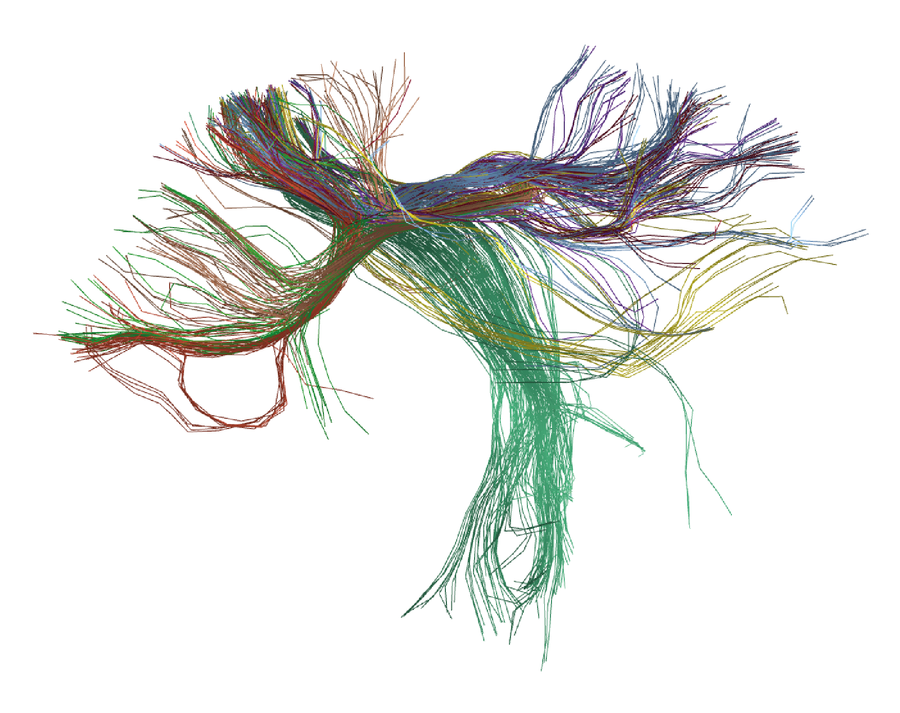
Figure 5. Results of applying HClust to the tractography dataset with 4000 streamlines from the HCP database. Eight clusters chosen manually are shown with random colors.
If you wish to run this example with the test dataset from the OpenNeuro database, we recommend using the brain tractography dataset consisting of 4,000 brain fibers ('subject_openneuro_4K.bundes/subject_openneuro_4K.bundesdata'),
defining distance thresholds as fiber_thr = 60 and partition_thr = 60.
Figure 6 displays the visualization results for clusters '0.bundles', '1.bundles', '2.bundles', '3.bundles', and '21.bundles'.
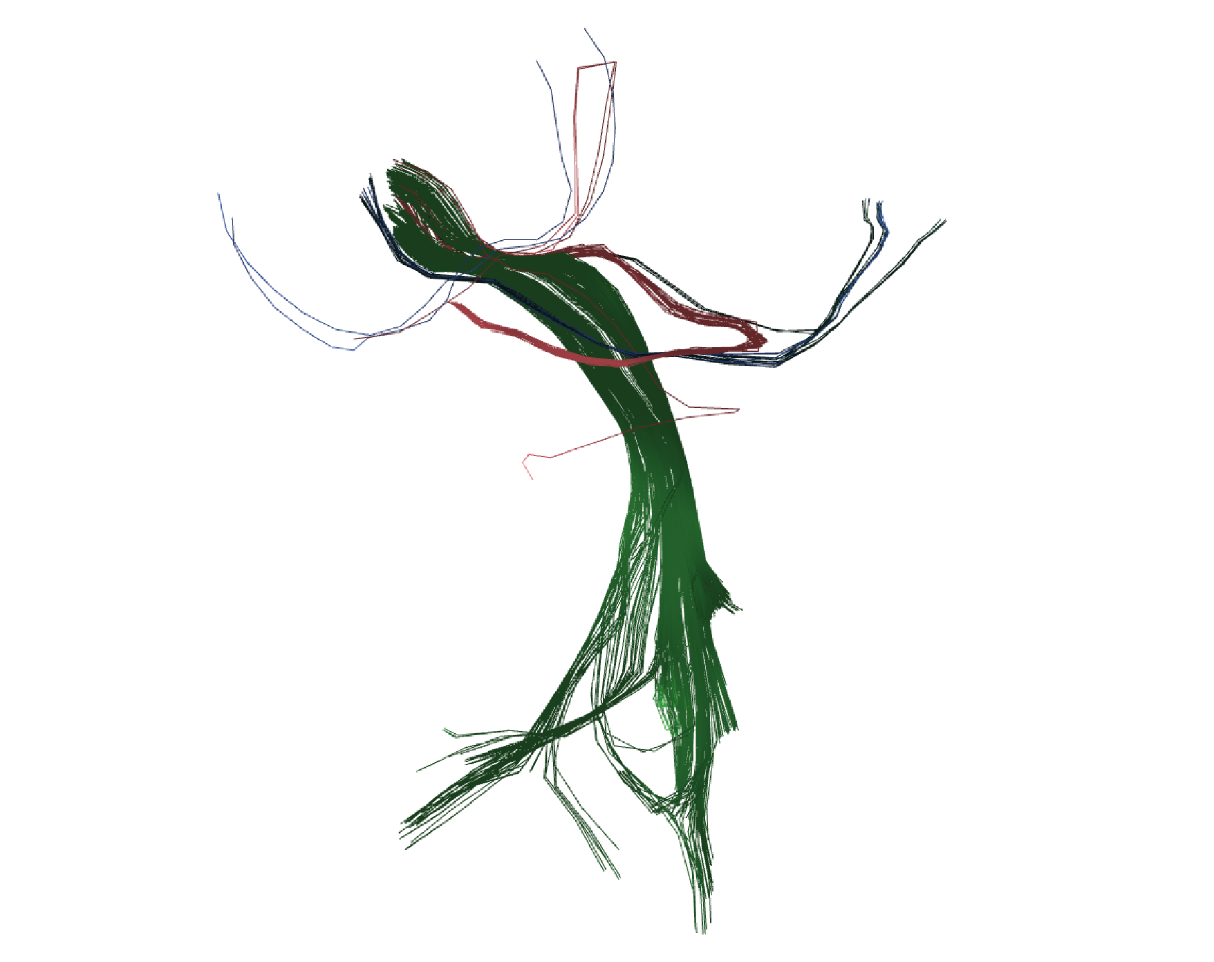
Figure 6. Results of applying HClust to the tractography dataset with 4000 streamlines from the OpenNeuro database. Five clusters, selected manually, are depicted with random colors.
FFClust
To execute FFClust, find on your computer the directory 'Downloads/testing_phybers/'. Afterward, open a Python terminal and run the following commands:
# Import the ffclust sub-module. Intra-subject clustering algorithm:
from phybers.clustering import ffclust

# Import the ffclust sub-module. Intra-subject clustering algorithm:
from phybers.utils import sampling

# Path to the tractography dataset file:
file_in = 'subject_15e5.bundles'

# Directory to save all segmentation results:
dir_out = 'ffclust_result'

# Indices of the points to be used in point K-means:
points = [0, 3, 10, 17, 20]

# Number of clusters to be computed for each point using K-Means:
ks = [200, 300, 300, 300, 200]

# Maximum distance threshold for the cluster reassignment in mm:
assign_thr = 6

# Maximum distance threshold for cluster merging in mm:
join_thr = 6

# Execute the ffclust function:
ffclust(file_in, dir_out, points, ks, assign_thr, join_thr)
Once FFClust has been successfully executed, in the directory 'Downloads/testing_phybers/ffclust_result/', you should be able to confirm the presence of the following outputs, that have the same structure as HClust:
'Downloads/testing_phybers/ffclust_result/final_bundles/': Directory that stores all the fiber clusters identified in separated datasets (bundles/bundlesdatafiles), sampled at 21 points. The file names are labeled with integer numbers ranging from zero to the total number of fiber clusters (N-1) identified.'Downloads/testing_phybers/ffclust_result/final_bundles_allpoints/': Directory that stores all the fiber clusters identified in separated datasets (bundles/bundlesdatafiles), with all points and in the original space. The file names are labeled with integer numbers ranging from zero to the total number of fiber clusters (N-1) identified.'Downloads/testing_phybers/ffclust_result/centroids/': A directory storing two files corresponding to a tractography dataset inbundles/bundlesdataformat, containing one centroid for each created cluster. This dataset is named'centroids.bundles/centroids.bundlesdata', and is sampled at 21 points in the atlas space (MNI).'Downloads/testing_phybers/ffclust_result/bundles_id.txt': Text file that stores the fiber indexes from the original input tractography dataset file for each detected cluster. Each line in the file correspond to a cluster in correlative order.'Downloads/testing_phybers/hclust_result/outputs/': Temporal directory with intermediate results, such as the point clusters.
Filtering the clusters with a size greater than 150 and a length in the range from 50 to 60 mm
The postprocessing() tool from the Utils module is useful for exploring and evaluating clustering and segmentation results.
This tool extracts information (metrics), such as cluster size (number of fibers), cluster mean length, and mean intra-cluster distance, from the generated clusters.
These results enable various analyses, such as the application of different filters to obtain clusters of a given size
or the construction of a histogram depicting the distribution of metrics.
In this example, we illustrate the usage of the PostProcessing sub-module applied to the results obtained with the ffclust() algorithm,
discussed in the previous subsection. First, the postprocessing() function is applied, returning a pandas.DataFrame object containing the following keys:
'size' (number of fibers in the bundle), 'len' (centroid length per bundle), and 'intra_mean' (mean intra-bundle Euclidean distance).
The DataFrame index corresponds to the cluster number; in other words, index zero of the DataFrame corresponds to cluster zero and centroid zero.
Next, a filtering criterion is applied, selecting clusters with a size greater or equal to 150, and a mean length between 50 and 60 mm. Next, the clusters meeting this condition are stored. Finally, a histogram is constructed to visualize the distribution of the selected clusters in relation to their size.
To execute this example, open the Python terminal in the 'Downloads/testing_phybers/' directory,
create a script named 'testing_postprocessing.py', copy the following command lines, and then run them.
# Import postprocessing:
from phybers.utils import postprocessing

# Import Python libraries for additional processing steps:
import numpy as np
import pandas as pd
import shutil
import os

# Set the input directory
dir_in = 'ffclust_result'

# Execute postprocessing:
df_metrics = postprocessing (dir_in)

# Save the DataFrame with calculated metrics
df_metrics.to_excel(os.path.join('ffclust_result', 'outputs', 'metrics.xlsx'))

# Filtering the clusters with a size greater than 150 and a length in the range from 50 to 60 mm:
filter_df_metrics = df_metrics[(df_metrics['size'] >= 150) & (df_metrics['len'] >= 50) & (df_metrics['len'] <= 60)]

# List with the indices of filtered fibers:
list_id_fibers_filter = list(filter_df_metrics.index)

# Define the output directory for filtered fibers:
directory = os.path.join('ffclust_result', 'filter_150S_50-60L')

# Create the directory if it doesn't exist:
if not os.path.exists(directory):
   os.mkdir(directory)

# # Copy the filtered fiber clusters to the created directory:
for i in list_id_fibers_filter:
   shutil.copy(os.path.join('ffclust_result', 'final_bundles_allpoints', str(i)+'.bundles'), os.path.join(directory, str(i)+'.bundles'))
   shutil.copy(os.path.join('ffclust_result', 'final_bundles_allpoints', str(i)+'.bundlesdata'), os.path.join(directory, str(i)+'.bundlesdata'))
In this example, the calculated DataFrame is automatically saved in the directory 'ffclust_result/outputs/' as an Excel file named 'metrics.xlsx'.
The DataFrame df_metrics is filtered and then the selected clusters are stored on the directory 'Downloads/testing_phybers/ffclust_result/filter_150S_50-60L/'.
Visualization of the filtered clusters
The filtered clusters are stored in the 'Downloads/testing_phybers/ffclust_result/filter_150S_50-60L/' directory.
To visualize them, run the graphical user interface of Fibervis using the following command lines and then drag all the bundles files.
This will allow you to obtain a visualization similar to the one shown in Figure 7.
# Import fibervis
from phybers.fibervis import start_fibervis

# Execute the graphical user interface for fibervis:
start_fibervis()
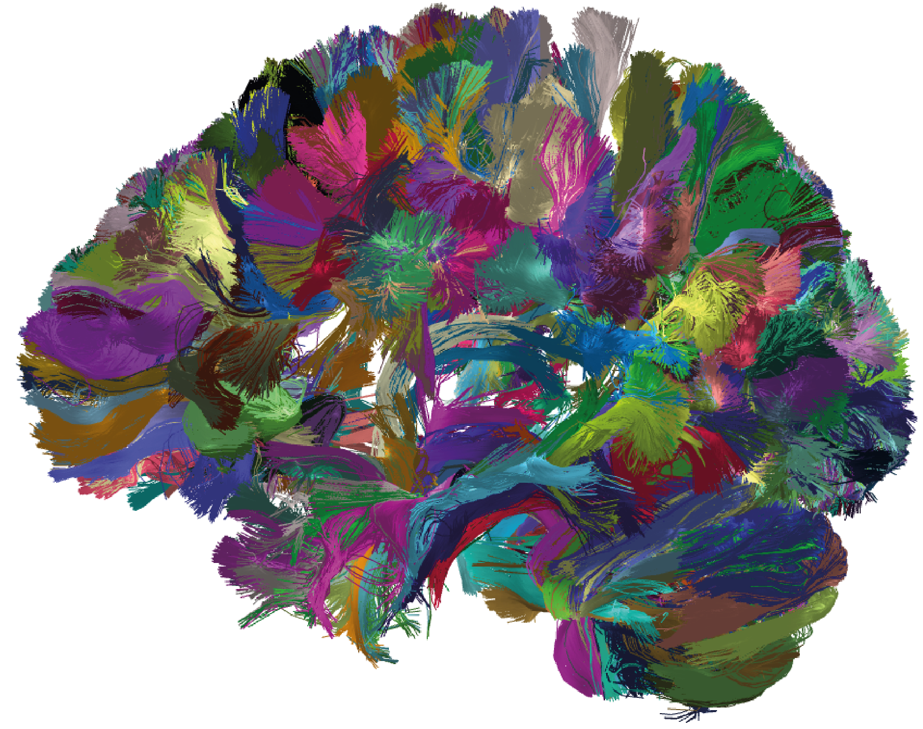
Figure 7. Results of applying FFClust to the whole-brain tractography dataset with 1.5 million streamlines from HCP database. The detected clusters were filtered using the PostProcessing sub-module of the Utils module; the filtering criterion shows clusters with a size greater than 150 and a mean length between 50 mm and 60 mm.
For the execution of the FFClust example using the OpenNeuro database (Test data download), begin by running the script provided in the preceding subsection (FFClust)
and configuring the 'file_in' argument as 'subject_openneuro_1M.bundes'.
Subsequently, run the script to filter clusters with a size greater than 150 and a mean length between 50 mm and 60 mm.
This process will enable you to achieve a visual representation similar to the one depicted in Figure 8.
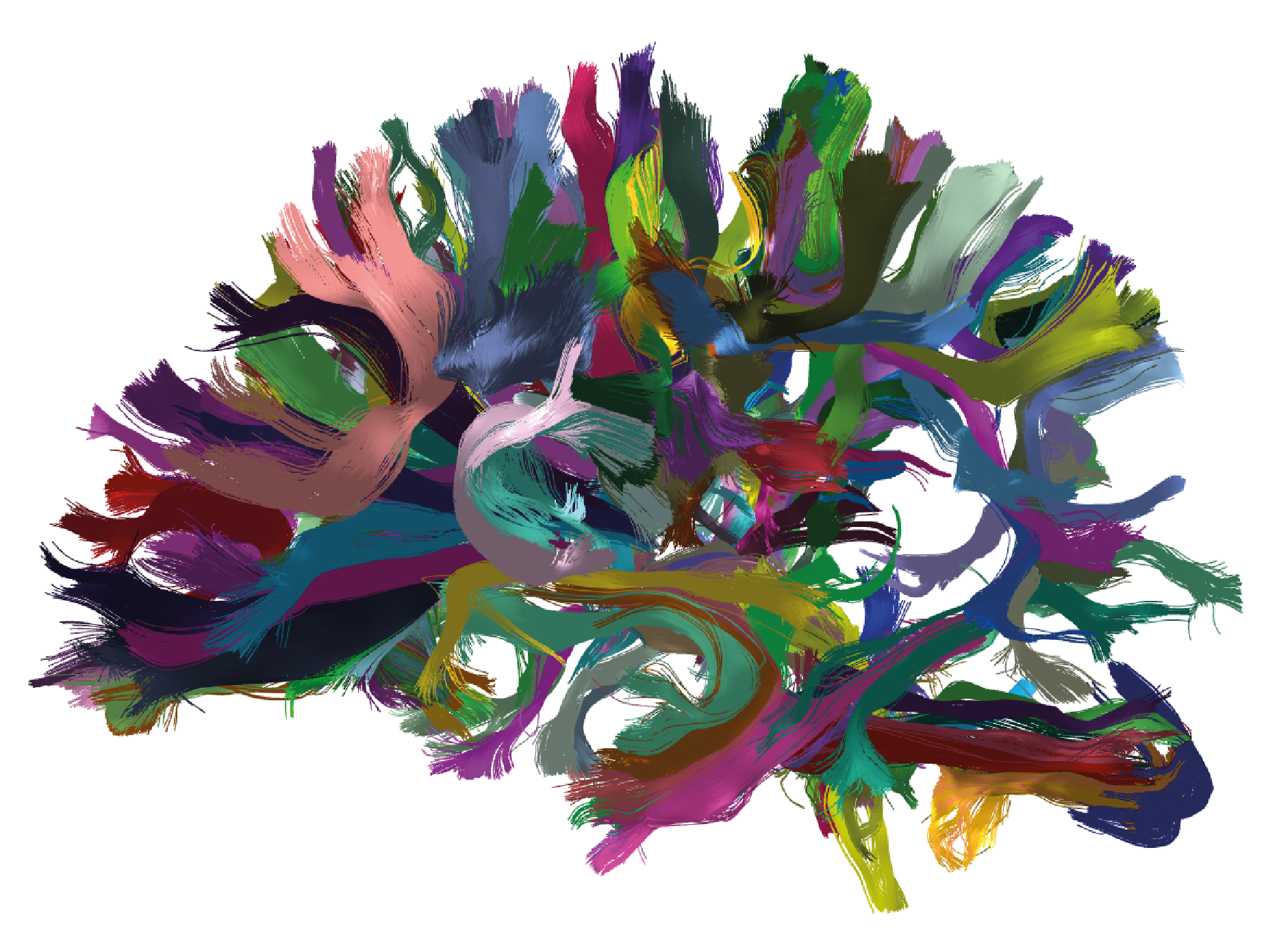
Figure 8. Results of applying FFClust to the whole-brain tractography dataset with 1 million streamlines from the OpenNeuro database. The detected clusters were filtered using the PostProcessing sub-module of the Utils module; the filtering criterion shows clusters with a size greater than 150 and a mean length between 50 mm and 60 mm.
Histogram of the filtered clusters
Below is an example that guides you through the process of calculating a histogram to analyse the size of the filtered clusters from the previous step.
To run the following command lines, create a script with the name 'testing_postprocessing_histogram.py'
in the 'testing_phybers/ffclust_result/' directory, save it, and then execute.
# Import Seaborn and Matplotlib for creating the histogram:
import seaborn as sns
import matplotlib.pyplot as plt

# Import the pandas library to handle data filtering:
import pandas as pd

# Import Python's os library for directory management:
import os

# Read the Excel file into a pandas DataFrame containing the calculated metrics for FFClust clusters:
df_metrics = pd.read_excel(os.path.join('ffclust_result', 'outputs', 'metrics.xlsx'))

# Filtering the clusters with a size greater than 150 and a length in the range from 50 to 60 mm:
filter_df_metrics = df_metrics[(df_metrics['size'] >= 150) & (df_metrics['len'] >= 50) & (df_metrics['len'] <= 60)]

# Set the bin width for the histogram:
bin_width = 100

# Find the maximum and minimum values of the 'size' column in the DataFrame:
max_lens = filter_df_metrics['size'].max()
min_lens = filter_df_metrics['size'].min()

# Create bins with the specified bin width, covering the range from the minimum to maximum 'size' values:
bins = range(min_lens, max_lens + bin_width, bin_width)

# Create a histogram plot using Seaborn, specifying the data, the 'size' column, bins, and visual settings:
sns.histplot(data=filter_df_metrics, x='size', bins=bins, kde=False, edgecolor='black')

# Set the title and labels for the plot:
plt.title('Clusters with a size greater than 150 and a length ranging from 50 to 60 mm')
plt.xlabel('Sizes')
plt.ylabel('Frequency')

# Adjust x-axis tick labels with rotation, alignment, and font size:
plt.xticks(bins, rotation=45, ha='right', fontsize=8)

# Add grid lines on the y-axis with a dashed linestyle and reduced alpha (transparency):
plt.grid(axis='y', linestyle='--', alpha=0.7)

# Display the histogram plot:
plt.show()
Figure 9 displays the expected result. It can be deduced that as the size of clusters for fibers with lengths between 50 and 60 mm increases, the number of fibers decreases.
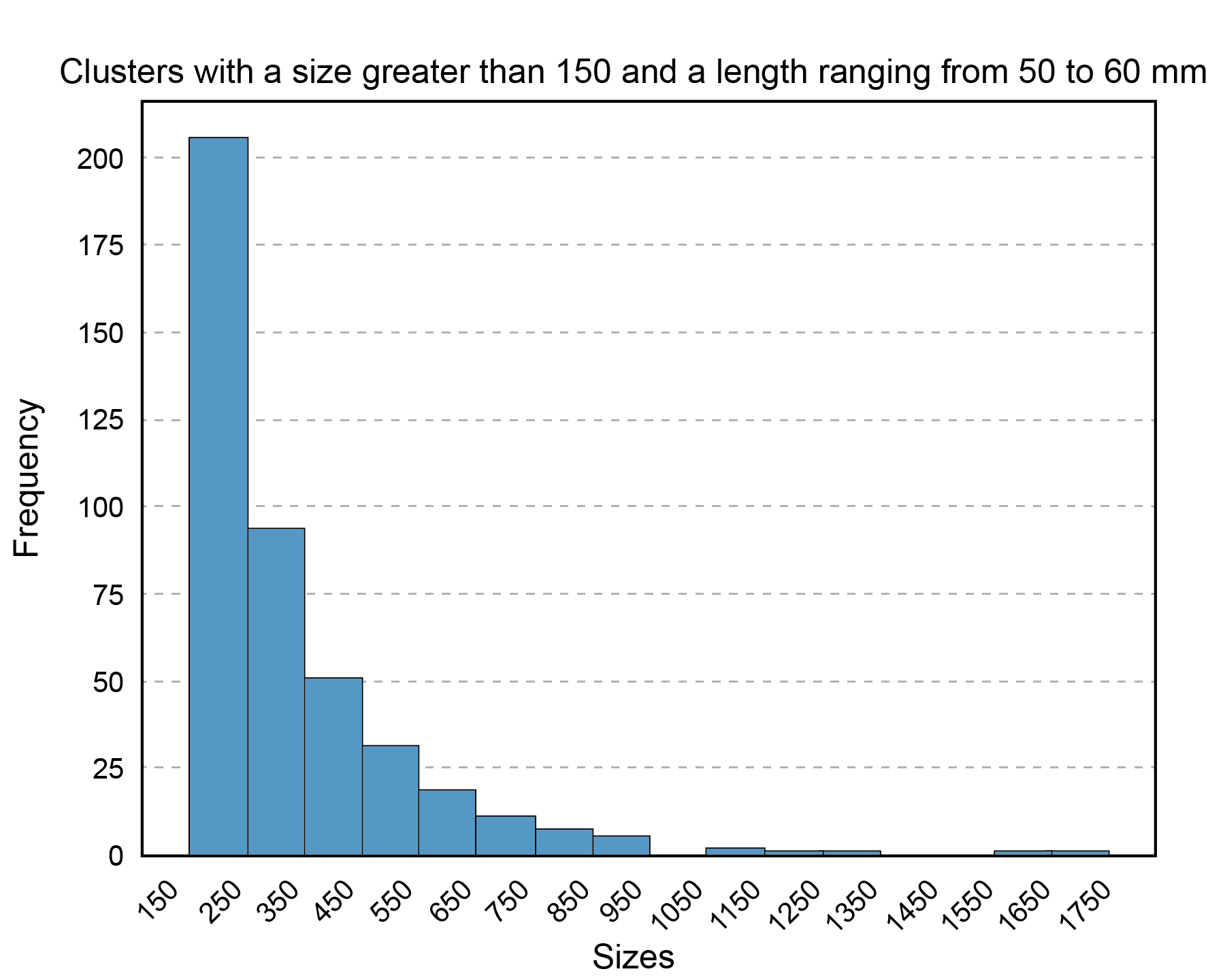
Figure 9. Histogram displaying the sizes of clusters obtained with FFClust that have a size greater than 150 and a length between 50 mm and 60 mm. On the x-axis, the cluster sizes are presented with 100-unit intervals in the range from 150 to 1750, while on the y-axis, the frequency or count of clusters is depicted according to their size.